6 Frequently Asked Questions
This chapter addresses questions that come up regularly on the GitHub issue tracker.
6.1 Sizing and responsive behavior
6.1.1 My plot is tiny in Shiny
Make sure opts_sizing(rescale = TRUE) is set (the default). When rescale = TRUE, the graphic scales to fill the available width while preserving its aspect ratio. If the plot still appears small, check that the girafeOutput() container has a reasonable width:
# UI
girafeOutput("plot", width = "100%")

# Server
output$plot <- renderGirafe({
  girafe(ggobj = gg, options = list(opts_sizing(rescale = TRUE)))
})
See Graphic size for a full explanation of aspect ratio vs. display size.
6.1.2 Extra whitespace below the plot
This usually happens when the container imposes a fixed height that is larger than the graphic needs. In responsive mode (rescale = TRUE), the height adjusts automatically to the width; any leftover vertical space appears as whitespace.
Solutions:
- In Shiny, leave
height = NULLingirafeOutput()so that the height follows the aspect ratio. - In flexdashboard or Quarto dashboards, make sure the card does not impose a fixed height. If it does, adjust
width_svg/height_svgso that the aspect ratio matches the container.
6.1.3 The plot does not fill a Quarto dashboard card
Quarto dashboard cards use a fill layout. Set both width and height to NULL in girafeOutput() so that the widget participates in the fill layout:
girafeOutput("plot", width = NULL, height = NULL)The widget will then expand to fill all available space in its parent container. See In Shiny for details on the three sizing modes.
6.1.4 How to control the plot size in R Markdown / Quarto documents
Leave width_svg and height_svg unset so that the knitr chunk options fig.width and fig.height are used automatically:
# ```{r fig.width=8, fig.height=5}
# girafe(ggobj = gg)
# ```
6.2 Tooltip issues
6.2.1 Special characters break tooltips
Characters such as single quotes ('), double quotes ("), angle brackets (<, >) and newlines in tooltip text can break the SVG markup.
Since version 0.8.0, ggiraph escapes these characters automatically. If you are on an older version, upgrade. If you still encounter an issue, make sure you are not injecting raw HTML through paste() or sprintf() without escaping.
6.2.2 I want HTML content in tooltips
Tooltips in ggiraph accept HTML. You can use tags such as <b>, <br>, <img>, <table>, etc. Build the HTML string in R and pass it as the tooltip aesthetic:
aes(tooltip = sprintf("<b>%s</b><br/>Value: %.1f", name, value))Be careful: the HTML is injected as-is, so sanitize any user-provided content to avoid breaking the SVG.
6.2.3 Tooltip order differs from bar order in stacked bar charts
Adding the tooltip aesthetic can change the implicit grouping that ggplot2 performs. This causes bars to be reordered or positions to break (e.g. position_jitterdodge no longer dodges correctly).
The fix is to explicitly set the group aesthetic so that ggplot2 ignores the interactive aesthetics when computing groups:
mapping = aes(tooltip = my_tooltip, group = interaction(factor1, factor2))The illustration below demonstrates the problem. The left plot specifies group = interaction(X, Group) explicitly — dodging works. The right plot omits group, so ggplot2 includes tooltip (which is unique per point) in the grouping, and dodging breaks:
library(patchwork)
set.seed(2)

data <- data.frame(
  X = sample(c("A", "B", "C"), 120, replace = TRUE),
  Y = rnorm(120),
  Group = sample(c("G1", "G2"), 120, replace = TRUE)
)

z1 <- ggplot(data, aes(x = X, y = Y, color = Group)) +
  geom_point_interactive(
    aes(tooltip = paste(Y), group = interaction(X, Group)),
    position = position_jitterdodge(jitter.width = 0, dodge.width = 0.8)) +
  labs(title = "correct graphic")

z2 <- ggplot(data, aes(x = X, y = Y, color = Group)) +
  geom_point_interactive(
    aes(tooltip = paste(Y)),
    position = position_jitterdodge(jitter.width = 0, dodge.width = 0.8)) +
  labs(title = "wrong graphic")

z1 + z2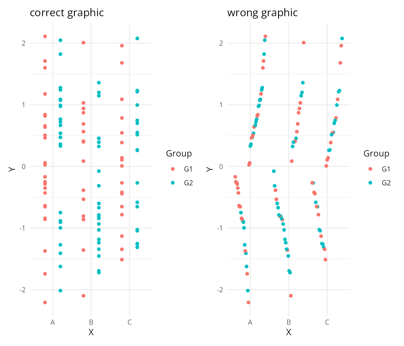
6.2.4 Tooltip does not appear on geom_boxplot_interactive
geom_boxplot_interactive() produces several sub-geometries (box, whiskers, median, outliers). The tooltip aesthetic applies to the box; outliers need separate attention. Provide tooltip inside aes(), not as a fixed parameter. If the tooltip still does not show, check that you have a recent version of ggiraph (>= 0.8.0).
6.2.5 Can I use after_stat() in the tooltip aesthetic?
Yes. Since ggiraph 0.8.10, after_stat() works in interactive aesthetics:
geom_bar_interactive(
  aes(tooltip = sprintf("count: %.0f", after_stat(count)))
)
If you get an error, make sure you are on the latest version of ggiraph.
6.3 Hover effects
6.3.1 Hover does not work
The data_id aesthetic is mandatory for hover effects. Without it, elements cannot be identified and no animation is applied:
# will NOT have hover effects
geom_point_interactive(aes(tooltip = name))

# WILL have hover effects
geom_point_interactive(aes(tooltip = name, data_id = name))
6.3.2 Elements with alpha = 0 do not react to hover
When alpha = 0 is set in the geom, the SVG element is rendered fully transparent. CSS hover styles (e.g. fill:yellow) cannot override the alpha channel set by the R graphics device.
Workaround: use a very small alpha value (alpha = 0.01) instead of 0. The element will be visually invisible but will still respond to mouse events.
6.3.3 Hover triggers in unexpected areas on line plots
When using geom_line_interactive() or geom_path_interactive(), you might notice that hover detection does not match the visible lines:
- Hover triggers even when the cursor is far from the line
- Placing the cursor on a line sometimes highlights a different one
- Other interactive elements located within areas “enclosed” by lines become inaccessible
The system treats lines as closed polygons instead of open paths. This creates polygon-shaped detection zones that encompass the area enclosed by the line segments.
Try it yourself: move your cursor around — hover zones don’t match the visible lines.
ggchick <- ggplot(
  data = ChickWeight,
  mapping = aes(
    y = weight,
    x = Time,
    color = factor(Diet),
    data_id = Chick)
) +
  geom_point_interactive(hover_nearest = TRUE) +
  geom_line_interactive(aes(group = Chick))

girafe(ggobj = ggchick)
Workaround 1 — disable hover_nearest (partial fix):
ggchick <- ggplot(
  data = ChickWeight,
  mapping = aes(
    y = weight,
    x = Time,
    color = factor(Diet),
    data_id = Chick)
) +
  geom_point_interactive(hover_nearest = FALSE) +
  geom_line_interactive(aes(group = Chick))

girafe(ggobj = ggchick)
Workaround 2 — use geom_segment_interactive() for precise control:
chick_weight_seg <- ChickWeight  |>
  as_tibble() |>
  arrange(Diet, Chick, Time) %>%
  group_by(Diet, Chick) %>%
  mutate(
    time_end = lead(Time),
    weight_end = lead(weight)
  ) %>%
  filter(!is.na(time_end))

ggchick <- ggplot(
  chick_weight_seg,
  mapping = aes(
    x = Time,
    y = weight,
    xend = time_end,
    yend = weight_end,
    data_id = Chick,
    tooltip = Diet,
    color = Diet
  )
) +
  geom_segment_interactive() +
  geom_point_interactive(hover_nearest = TRUE)

girafe(ggobj = ggchick, options = list(opts_sizing(rescale = TRUE)))
6.3.4 How to highlight the hovered element and dim the others
Use opts_hover_inv() to reduce the opacity of non-hovered elements:
girafe(
  ggobj = gg,
  options = list(
    opts_hover(css = "stroke-width:2;"),
    opts_hover_inv(css = "opacity:0.1;")
  )
)
6.3.5 opts_hover() does not seem to work
If you upgraded from a version before 0.8.0, note that the old hover_css argument in girafe() has been replaced by opts_hover(css = ...) passed via the options list. The old syntax is no longer supported.
# Old (no longer works)
girafe(ggobj = gg, hover_css = "fill:red;")

# Current
girafe(ggobj = gg, options = list(opts_hover(css = "fill:red;")))
6.4 Fonts and text rendering
6.4.1 Text looks different after deployment
When you deploy to shinyapps.io, a Linux server, or a Docker container, the fonts available on the server are likely different from your local machine. The SVG references font names, and if the font is not found, the browser falls back to a generic family (often a serif font).
Solutions:
Use a web font (recommended): register it with
gdtools::register_gfont()for the R device, and embed it in the HTML output for the browser. See Fonts management for full instructions.Use Liberation Sans for an offline alternative that does not require internet access:
library(gdtools)
register_liberationsans()
girafe(
  ggobj = gg,
  dependencies = list(gdtools::liberationsansHtmlDependency())
)- Validate your fonts during development with
check_fonts_registered = TRUEandcheck_fonts_dependencies = TRUEingirafe()to catch issues early. See Font validation.
6.4.2 “fontconfig error: unable to match font pattern”
This error occurs on Linux/macOS systems where the requested font is not installed. Install the font at the OS level, or use register_gfont() / register_liberationsans() from the gdtools package.
6.4.3 Y-axis labels are misaligned
This is almost always a font issue. The R graphics device uses font metrics to position text. If the font available on the production server differs from the one used locally, positions shift. The fix is to ensure the same font is used everywhere (see above).
6.4.4 Downloaded PNG has wrong fonts
The “save as PNG” button in the toolbar renders the SVG in the browser. If the font is not available in the browser, it falls back to a default. Embed the font as an HTML dependency so the browser can use it for the PNG export too.
6.5 Shiny integration
6.5.1 How to get the selected element values
Selections are available as reactive values. The naming convention is input$<outputId>_selected for panel selections:
# UI
girafeOutput("plot")

# Server
observeEvent(input$plot_selected, {
  cat("Selected:", input$plot_selected, "\n")
})
Legend and theme selections use _key_selected and _theme_selected respectively. See Shiny and ggiraph reactive values for details.
6.5.2 How to clear selections programmatically
Send an empty character vector via session$sendCustomMessage:
session$sendCustomMessage(type = "plot_set", message = character(0))6.5.3 The outputId must not contain dots
girafeOutput("my.plot") will silently fail because the JavaScript handler uses the id as part of a message type name. Use underscores instead: girafeOutput("my_plot").
6.6 Quarto, R Markdown and Flexdashboard
6.6.1 ggiraph does not render inside a loop
In R Markdown / Quarto, girafe() must be printed to produce output. Inside a loop, wrap the call in print() or collect the widgets in a list:
for (i in 1:3) {
  gg <- ggplot(mtcars, aes(wt, mpg)) +
    geom_point_interactive(aes(tooltip = row.names(mtcars), data_id = row.names(mtcars)))
  print(girafe(ggobj = gg))
}
Alternatively, use htmltools::tagList() to emit all widgets at once.
6.7 Toolbar and export
6.8 Zoom and pan
6.8.1 Zoom does not activate automatically
By default, the user must click the toolbar button to activate zoom. Set default_on = TRUE to activate it on load:
girafe(
  ggobj = gg,
  options = list(opts_zoom(max = 5, default_on = TRUE))
)
6.8.2 Axis labels disappear when zooming
This is expected: when you pan away from the axis area, the axis labels leave the viewport. The SVG viewbox clips content outside the visible area. There is no option to keep axes pinned during zoom.
6.9 Accessibility
6.9.1 How to add alt text to a girafe graphic
In a Quarto / R Markdown document, use the fig-alt chunk option:
# ```{r}
# #| fig-alt: "Scatter plot of engine displacement vs. city fuel economy"
# girafe(ggobj = gg)
```
In Shiny, you can add a title and description via the SVG attributes using the desc and title arguments:
girafe(ggobj = gg, desc = "Scatter plot description", title = "My plot")