Clinical Tables with ‘flextable’, ‘tables’ and ‘rtables’

‘flextable’ package

The primary goal of ‘flextable’(Gohel and Skintzos 2023, website) is to provide a versatile and efficient solution for creating and formatting tables in R.

It aims to make table creation and customization easier by offering a flexible and user-friendly interface within the R environment. The package offers extensive capabilities for creating table structure, format content, and appearance.

ft <- summarizor(cars) |> 
  as_flextable(sep_w=0) |> 
  color(i = ~stat == "range", 
        color = "pink") |> 
  bold(j = 1) |> 
  italic(j = 2, italic = TRUE)

Statistic
(N=50)

speed

Mean (SD)

15.4 (5.3)

Median (IQR)

15.0 (7.0)

Range

4.0 - 25.0

dist

Mean (SD)

43.0 (25.8)

Median (IQR)

36.0 (30.0)

Range

2.0 - 120.0

features: quick overview

with flextable()

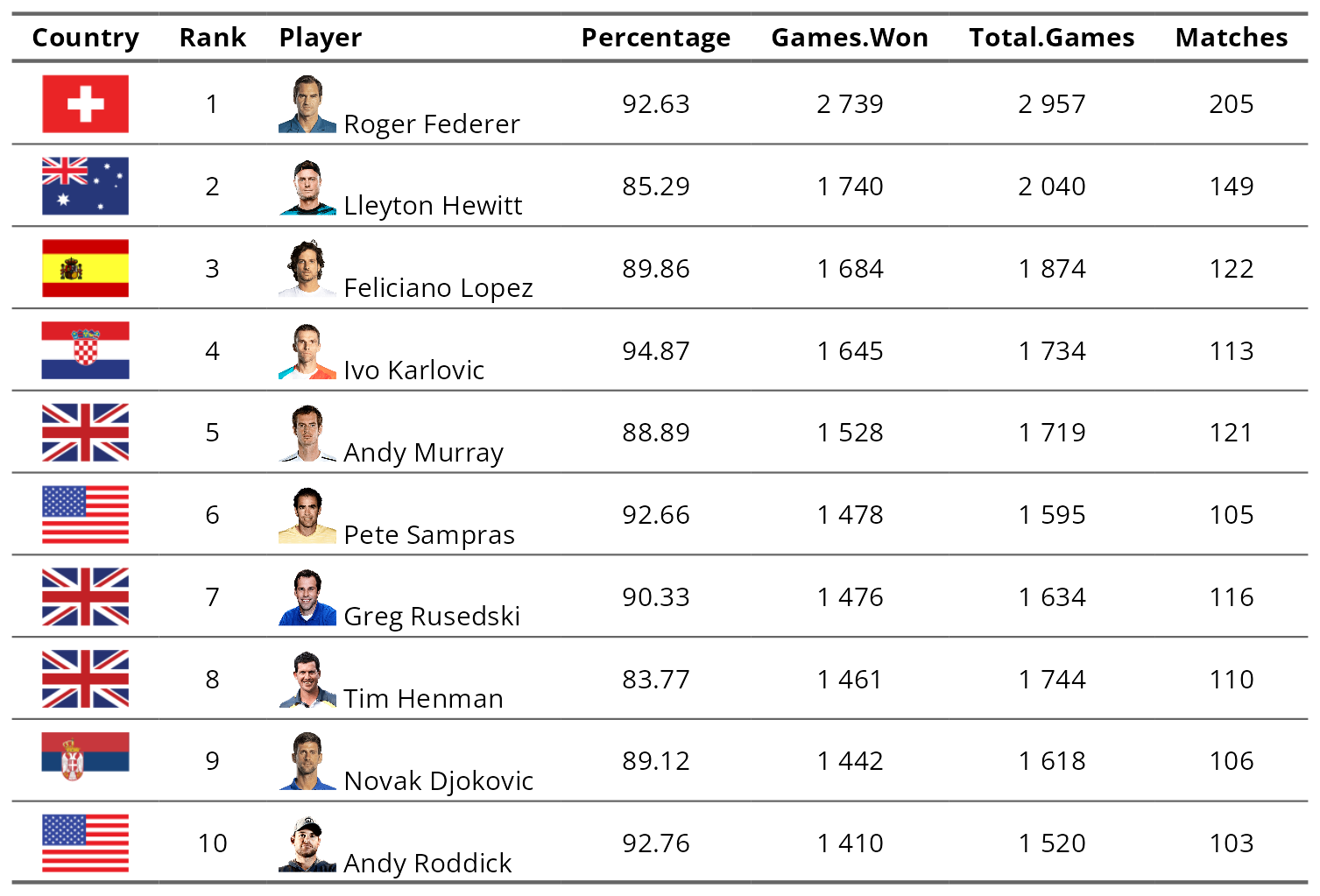
‘flextable’ can easily create reporting table from data.frame. You can merge cells, add header rows or specify how data should be displayed in cells.

tennis-players as png

with as_flextable()

The as_flextable() function is used to transform specific objects into flextable objects.

with(palmerpenguins::penguins, table(species, island)) |>
  as_flextable()

species

island

Biscoe

Dream

Torgersen

Total

Adelie

Count

44 (12.8%)

56 (16.3%)

52 (15.1%)

152 (44.2%)

Mar. pct (1)

26.2% ; 28.9%

45.2% ; 36.8%

100.0% ; 34.2%

Chinstrap

Count

0 (0.0%)

68 (19.8%)

0 (0.0%)

68 (19.8%)

Mar. pct

0.0% ; 0.0%

54.8% ; 100.0%

0.0% ; 0.0%

Gentoo

Count

124 (36.0%)

0 (0.0%)

0 (0.0%)

124 (36.0%)

Mar. pct

73.8% ; 100.0%

0.0% ; 0.0%

0.0% ; 0.0%

Total

Count

168 (48.8%)

124 (36.0%)

52 (15.1%)

344 (100.0%)

(1) Columns and rows percentages

Supported outputs

It supports various output formats to meet different needs :

Demographic table example

adsl <- select(formatters::ex_adsl, AGE, SEX, ARM)
col_labels <- map_chr(adsl, function(x) attr(x, "label"))
summarizor(adsl, by = "ARM") |> 
  as_flextable()

A: Drug X
(N=134)

B: Placebo
(N=134)

C: Combination
(N=132)

AGE

Mean (SD)

33.8 (6.6)

35.4 (7.9)

35.4 (7.7)

Median (IQR)

33.0 (11.0)

35.0 (10.0)

35.0 (10.0)

Range

21.0 - 50.0

21.0 - 62.0

20.0 - 69.0

SEX

F

79 (58.96%)

77 (57.46%)

66 (50.00%)

M

51 (38.06%)

55 (41.04%)

60 (45.45%)

U

3 (2.24%)

2 (1.49%)

4 (3.03%)

UNDIFFERENTIATED

1 (0.75%)

0 (0.00%)

2 (1.52%)

Visual aspect can be improved:

  • by using options of as_flextable(),
  • by adding tabulations with prepend_chunks(),
  • by using proper labels with labelizor().
ft <- summarizor(adsl, by = "ARM") |>
  as_flextable(sep_w = 0, separate_with = "variable", 
               spread_first_col = TRUE) |>
  align(i = ~ !is.na(variable), align = "left") |> 
  prepend_chunks(i = ~ is.na(variable), j  ="stat", 
                 as_chunk("\t")) |> 
  labelizor(j = c("stat"), labels = col_labels, 
            part = "all") |> 
  autofit()
ft

A: Drug X
(N=134)

B: Placebo
(N=134)

C: Combination
(N=132)

Age

Mean (SD)

33.8 (6.6)

35.4 (7.9)

35.4 (7.7)

Median (IQR)

33.0 (11.0)

35.0 (10.0)

35.0 (10.0)

Range

21.0 - 50.0

21.0 - 62.0

20.0 - 69.0

Sex

F

79 (58.96%)

77 (57.46%)

66 (50.00%)

M

51 (38.06%)

55 (41.04%)

60 (45.45%)

U

3 (2.24%)

2 (1.49%)

4 (3.03%)

UNDIFFERENTIATED

1 (0.75%)

0 (0.00%)

2 (1.52%)

Save result in a file

You can quickly save the result:

  • in a Microsoft Word with save_as_docx(),
  • in a Microsoft PowerPoint with save_as_pptx(),
  • in a PNG with save_as_image() with full support for fonts.
save_as_docx(ft, 
  path = "assets/files/ft.docx")
save_as_pptx(ft,
  path = "assets/files/ft.pptx")
save_as_image(ft,
  path = "assets/files/ft.png")

You can use package ‘doconv’ to produce miniatures from ‘Word’, ‘PowerPoint’ or ‘PDF’ files.

doconv::to_miniature("assets/files/ft.docx", fileout = "assets/files/ft-docx.png")

R Tables for Regulatory Submissions Working Group

https://rconsortium.github.io/rtrs-wg/

The goal of the working group is to create standards for creating tables that meet the requirements of FDA submission documents, and hence enhance the suitability of R for FDA submissions. […]

Participation in the working group led to several advances in clinical reporting with ‘flextable’.

Two types of table packages

Focused on formatting, with content definition populated from a data.frame (‘flextable’, ‘gt’). The data.frame based approach of ‘flextable’ requires to first build a data.frame that contains all data and then to format it.

data.frame based approach

It sometimes results in code that is too long and painful to write in order to produce the tables in the book.

package

ASCII

PDF

HTML

DOCX

RTF

PPTX

GRID

flextable

Focused on functional expression and content definition, with little visual formatting capability (‘tables’, ‘rtables’, ‘tfrmt’, ‘tidytlg’). Packages ‘tables’ and ‘rtables’ are expressive enough to allow these tables to be formulated and can be converted to flextable.

as_flextable approach

Use ‘tables’(Murdoch 2023, website) and get a flextable with as_flextable() function.

Use ‘rtables’(Becker and Waddell 2023, website) and get a flextable with tt_to_flextable() function.

package

ASCII

PDF

HTML

DOCX

RTF

PPTX

GRID

rtables

tables

Disposition table

This table taken from the book shows the data.frame approach with flextable.

Disposition table preparation

Function tabulator() is used to prepare/structure the table.

The very first step is to create the data.frame that will be used by function tabulator() (40 lines of code with tidyverse).

TRT01A

EOSSTT

DCSREAS

n

percent

factor

factor

factor

integer

numeric

A: Drug X

COMPLETED

68

0.5

B: Placebo

COMPLETED

66

0.5

C: Combination

COMPLETED

73

0.6

A: Drug X

ONGOING

24

0.2

B: Placebo

ONGOING

28

0.2

C: Combination

ONGOING

21

0.2

A: Drug X

DISCONTINUED

ADVERSE EVENT

3

0.0

A: Drug X

DISCONTINUED

DEATH

25

0.2

A: Drug X

DISCONTINUED

LACK OF EFFICACY

2

0.0

A: Drug X

DISCONTINUED

PHYSICIAN DECISION

2

0.0

n: 47

tab <- tabulator(
  x = dat,
  rows = c("EOSSTT", "DCSREAS"), 
  columns = "TRT01A",
  content_cell = 
    as_paragraph(
      fmt_n_percent(n, percent)
    )
)

Disposition table creation

ft <- as_flextable(tab,
  spread_first_col = TRUE,
  columns_alignment = "center"
)

# add '(N=xx)'
TRT_COUNTS <- setNames(
  part_header$n_part,
  part_header$TRT01A
)
for (TRT_COD in names(TRT_COUNTS)) {
  ft <- append_chunks(
    x = ft, part = "header", i = 1,
    j = tabulator_colnames(
      tab,
      columns = "content_cell",
      TRT01A %in% !!TRT_COD
    ),
    as_chunk(TRT_COUNTS[TRT_COD],
      formatter = function(n) sprintf("\n(N=%.0f)", n)
    )
  )
}

ft <- labelizor(ft,
  j = "DCSREAS",
  part = "all", labels = function(x) tools::toTitleCase(tolower(x))
) |>
  labelizor(
    labels = c(Dcsreas = ""),
    j = "DCSREAS", part = "header"
  ) |>
  align(
    i = ~ !is.na(EOSSTT) | seq_along(EOSSTT) == 1,
    j = 1, align = "left"
  ) |>
  prepend_chunks(
    i = ~ is.na(EOSSTT),
    j = "DCSREAS", as_chunk("\t")
  ) |>
  autofit()

A: Drug X
(N=134)

B: Placebo
(N=134)

C: Combination
(N=132)

Completed

68 (50.7%)

66 (49.3%)

73 (55.3%)

Ongoing

24 (17.9%)

28 (20.9%)

21 (15.9%)

Discontinued

Adverse Event

3 (2.2%)

6 (4.5%)

5 (3.8%)

Death

25 (18.7%)

23 (17.2%)

22 (16.7%)

  Adverse Event

9 (6.7%)

7 (5.2%)

10 (7.6%)

  Disease Progression

8 (6.0%)

6 (4.5%)

6 (4.5%)

  Lost to Follow Up

2 (1.5%)

2 (1.5%)

2 (1.5%)

  Missing

2 (1.5%)

3 (2.2%)

2 (1.5%)

  Post-Study Reporting of Death

1 (0.7%)

2 (1.5%)

1 (0.8%)

  Suicide

2 (1.5%)

2 (1.5%)

1 (0.8%)

  Unknown

1 (0.7%)

1 (0.7%)

Lack of Efficacy

2 (1.5%)

2 (1.5%)

3 (2.3%)

Physician Decision

2 (1.5%)

3 (2.2%)

2 (1.5%)

Protocol Violation

5 (3.7%)

3 (2.2%)

4 (3.0%)

Withdrawal by Parent/Guardian

4 (3.0%)

2 (1.5%)

1 (0.8%)

Withdrawal by Subject

1 (0.7%)

1 (0.7%)

1 (0.8%)

Adverse Event Table

This table is using package tables::tabular() to produce a tabular object that will then be transformed into a flextable with function as_flextable().

Adverse Event Table preparation

link: https://rconsortium.github.io/rtrs-wg/commontables.html#tables-5

heading <- tabular(
  Heading("")*1*
    Heading("")*count ~ 
    Heading()*ARM, data = ex_adsl)

body <- tabular( 
  Heading("Patients with at least one event")*1*
    Heading("")*countpercentid*Arguments(ARM = ARM)*
    Heading()*USUBJID +
    
  Heading("Total number of events")*1*Heading("")*1 +
    
  Heading()*AEBODSYS*
    (Heading("Patients with at least one event")*
       Percent(denom = ARM, fn = countpercentid)*
       Heading()*USUBJID +
     Heading("Total number of events")*1 +
     Heading()*AEDECOD*DropEmpty(which = "row")*
       Heading()*Percent(denom = ARM, fn = countpercentid)*
       Heading()*USUBJID) ~ 
    
  Heading()*ARM, 
  data = ex_adae)
tab <- rbind(heading, body)

console output for tab

Adverse Event Table creation

‘flextable’ code: https://rconsortium.github.io/rtrs-wg/commontables.html#flextable-5

ae_ft <- as_flextable(
  body,
  spread_first_col = TRUE,
  add_tab = TRUE) |>
  align(
    j = 1, part = "all",
    align = "left") |>
  add_header_row(
    values = 
      c("", fmt_header_n(subject_counts,
                         newline = FALSE)),
    top = FALSE) |> 
  hline(
    i = 1,
    part = "header", 
    border = fp_border_default(width = 0))

A: Drug X

B: Placebo

C: Combination

(N=134)

(N=134)

(N=132)

Patients with at least one event

122 (91.04%)

123 (91.79%)

120 (90.91%)

Total number of events

609

622

703

cl A.1

Patients with at least one event

78 (58.21%)

75 (55.97%)

89 (66.42%)

Total number of events

132

130

160

dcd A.1.1.1.1

50 (37.31%)

45 (33.58%)

63 (47.01%)

dcd A.1.1.1.2

48 (35.82%)

48 (35.82%)

50 (37.31%)

cl B.1

Patients with at least one event

47 (35.07%)

49 (36.57%)

43 (32.09%)

Total number of events

56

60

62

dcd B.1.1.1.1

47 (35.07%)

49 (36.57%)

43 (32.09%)

cl B.2

Patients with at least one event

79 (58.96%)

74 (55.22%)

85 (63.43%)

Total number of events

129

138

143

dcd B.2.1.2.1

49 (36.57%)

44 (32.84%)

52 (38.81%)

dcd B.2.2.3.1

48 (35.82%)

54 (40.30%)

51 (38.06%)

cl C.1

Patients with at least one event

43 (32.09%)

46 (34.33%)

43 (32.09%)

Total number of events

55

63

64

dcd C.1.1.1.3

43 (32.09%)

46 (34.33%)

43 (32.09%)

cl C.2

Patients with at least one event

35 (26.12%)

48 (35.82%)

55 (41.04%)

Total number of events

48

53

65

dcd C.2.1.2.1

35 (26.12%)

48 (35.82%)

55 (41.04%)

cl D.1

Patients with at least one event

79 (58.96%)

67 (50.00%)

80 (59.70%)

Total number of events

127

106

135

dcd D.1.1.1.1

50 (37.31%)

42 (31.34%)

51 (38.06%)

dcd D.1.1.4.2

48 (35.82%)

42 (31.34%)

50 (37.31%)

cl D.2

Patients with at least one event

47 (35.07%)

58 (43.28%)

57 (42.54%)

Total number of events

62

72

74

dcd D.2.1.5.3

47 (35.07%)

58 (43.28%)

57 (42.54%)

Concomitant Medications Table

This table is using package ‘rtables’ to produce an object that will then be transformed into a flextable with function rtables::tt_to_flextable().

Concomitant Medications preparation

link: https://rconsortium.github.io/rtrs-wg/commontables.html#rtables-7

lyt <- basic_table(
  show_colcounts = TRUE) |>
  split_cols_by("TRT01A") |>
  analyze("EOSSTT", top_afun) |>
  split_rows_by("EOSSTT",
    split_fun = 
      keep_split_levels("DISCONTINUED")
  ) |>
  analyze("DCSREAS", count_pct_afun) |>
  split_rows_by("DCSREAS",
    split_fun = 
      keep_split_levels("DEATH")
  ) |>
  analyze("DTHCAUS", count_pct_afun)

tab <- build_table(lyt, adsl)
                                  A: Drug X    B: Placebo   C: Combination
                                   (N=134)      (N=134)        (N=132)    
——————————————————————————————————————————————————————————————————————————
Completed                         68 (50.7%)   66 (49.3%)     73 (55.3%)  
Ongoing                           24 (17.9%)   28 (20.9%)     21 (15.9%)  
DISCONTINUED                                                              
  ADVERSE EVENT                    3 (2.2%)     6 (4.5%)       5 (3.8%)   
  DEATH                           25 (18.7%)   23 (17.2%)     22 (16.7%)  
  LACK OF EFFICACY                 2 (1.5%)     2 (1.5%)       3 (2.3%)   
  PHYSICIAN DECISION               2 (1.5%)     3 (2.2%)       2 (1.5%)   
  PROTOCOL VIOLATION               5 (3.7%)     3 (2.2%)       4 (3.0%)   
  WITHDRAWAL BY PARENT/GUARDIAN    4 (3.0%)     2 (1.5%)       1 (0.8%)   
  WITHDRAWAL BY SUBJECT            1 (0.7%)     1 (0.7%)       1 (0.8%)   
DEATH                                                                     
  ADVERSE EVENT                    9 (6.7%)     7 (5.2%)      10 (7.6%)   
  DISEASE PROGRESSION              8 (6.0%)     6 (4.5%)       6 (4.5%)   
  LOST TO FOLLOW UP                2 (1.5%)     2 (1.5%)       2 (1.5%)   
  MISSING                          2 (1.5%)     3 (2.2%)       2 (1.5%)   
  Post-study reporting of death    1 (0.7%)     2 (1.5%)       1 (0.8%)   
  SUICIDE                          2 (1.5%)     2 (1.5%)       1 (0.8%)   
  UNKNOWN                          1 (0.7%)     1 (0.7%)       0 (0.0%)   

Concomitant Medications creation

ft <- tt_to_flextable(tab) |> 
  theme_booktabs() |> 
  font(fontname = "Open Sans") |> 
  bold(i = ~ V2 %in% "", 
       j = 1, bold = TRUE) |> 
  bold(i = 1, j = 1, 
       bold = TRUE) |> 
  align(j = 2:4, align = "center", 
        part = "all") |> 
  set_table_properties(layout = "fixed") |> 
  autofit()

Fonts, table layout and few other details need to be changed to produce a nice flextable.

A: Drug X

B: Placebo

C: Combination

(N=134)

(N=134)

(N=132)

Completed

68 (50.7%)

66 (49.3%)

73 (55.3%)

Ongoing

24 (17.9%)

28 (20.9%)

21 (15.9%)

DISCONTINUED

ADVERSE EVENT

3 (2.2%)

6 (4.5%)

5 (3.8%)

DEATH

25 (18.7%)

23 (17.2%)

22 (16.7%)

LACK OF EFFICACY

2 (1.5%)

2 (1.5%)

3 (2.3%)

PHYSICIAN DECISION

2 (1.5%)

3 (2.2%)

2 (1.5%)

PROTOCOL VIOLATION

5 (3.7%)

3 (2.2%)

4 (3.0%)

WITHDRAWAL BY PARENT/GUARDIAN

4 (3.0%)

2 (1.5%)

1 (0.8%)

WITHDRAWAL BY SUBJECT

1 (0.7%)

1 (0.7%)

1 (0.8%)

DEATH

ADVERSE EVENT

9 (6.7%)

7 (5.2%)

10 (7.6%)

DISEASE PROGRESSION

8 (6.0%)

6 (4.5%)

6 (4.5%)

LOST TO FOLLOW UP

2 (1.5%)

2 (1.5%)

2 (1.5%)

MISSING

2 (1.5%)

3 (2.2%)

2 (1.5%)

Post-study reporting of death

1 (0.7%)

2 (1.5%)

1 (0.8%)

SUICIDE

2 (1.5%)

2 (1.5%)

1 (0.8%)

UNKNOWN

1 (0.7%)

1 (0.7%)

0 (0.0%)

Pagination

The pagination of tables allows you to control their position in relation to page breaks. Packages ‘tables’, ‘rtables’ and ‘flextable’ implement their pagination vision.

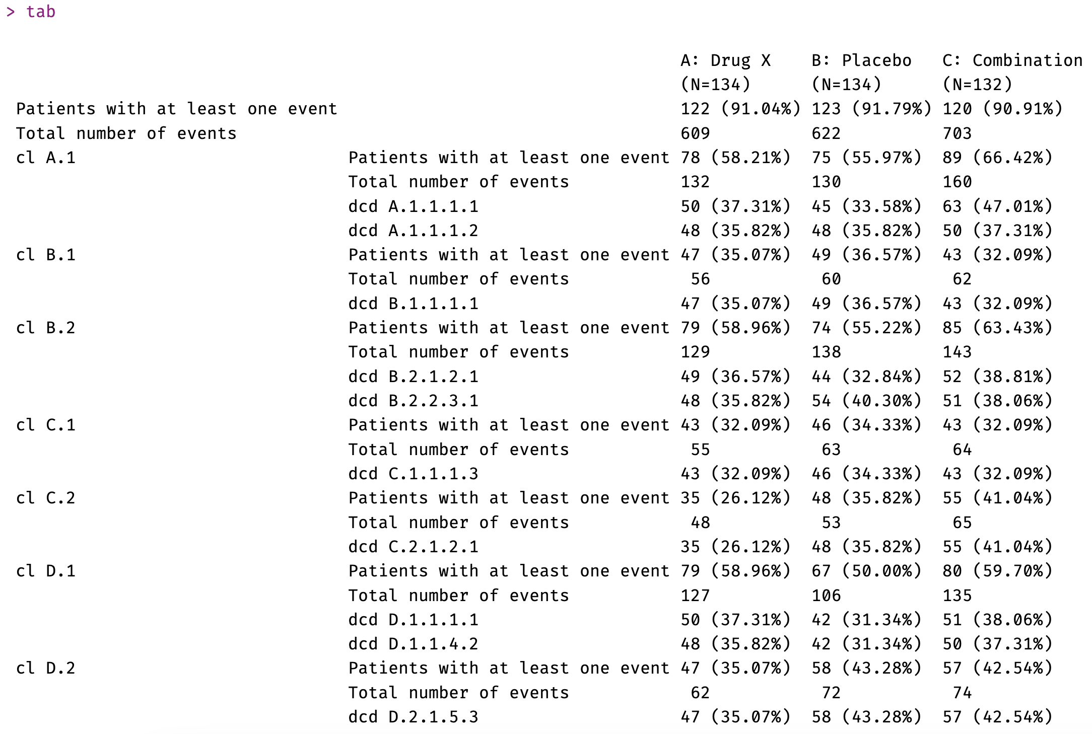
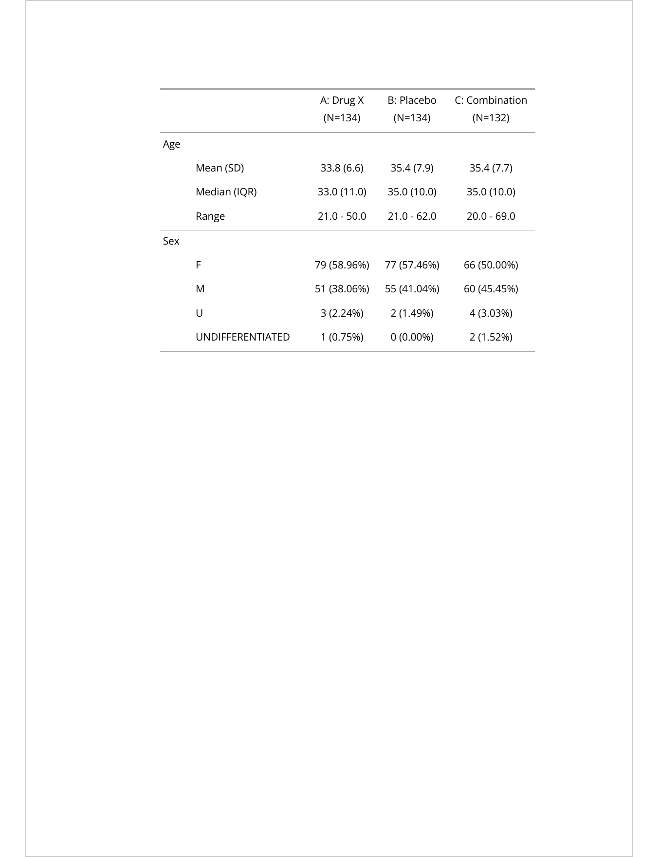
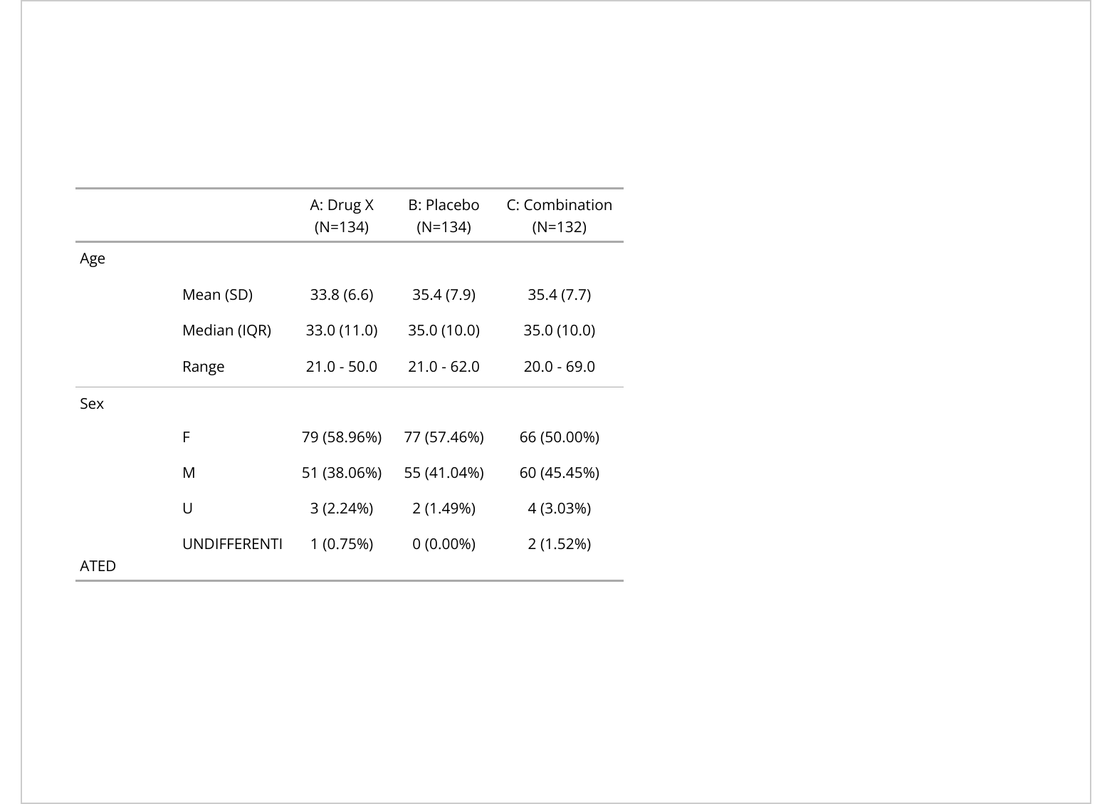
Pagination with ‘flextable’

When working with Word or RTF, it is possible to prevents breaks between tables rows you want to stay together. Function paginate() let you define this pagination.

From https://ardata-fr.github.io/flextable-book/layout.html#pagination

ft_2 <- tabular(
  cut * clarity ~ Format(digits = 2) *
    (x + y) * (mean + sd),
  data = dat
) |> ... |> 
  paginate(
    init = TRUE, 
    group = "COL1",
    group_def = "nonempty")

example_tabular_paginated.docx

paginated table in Word

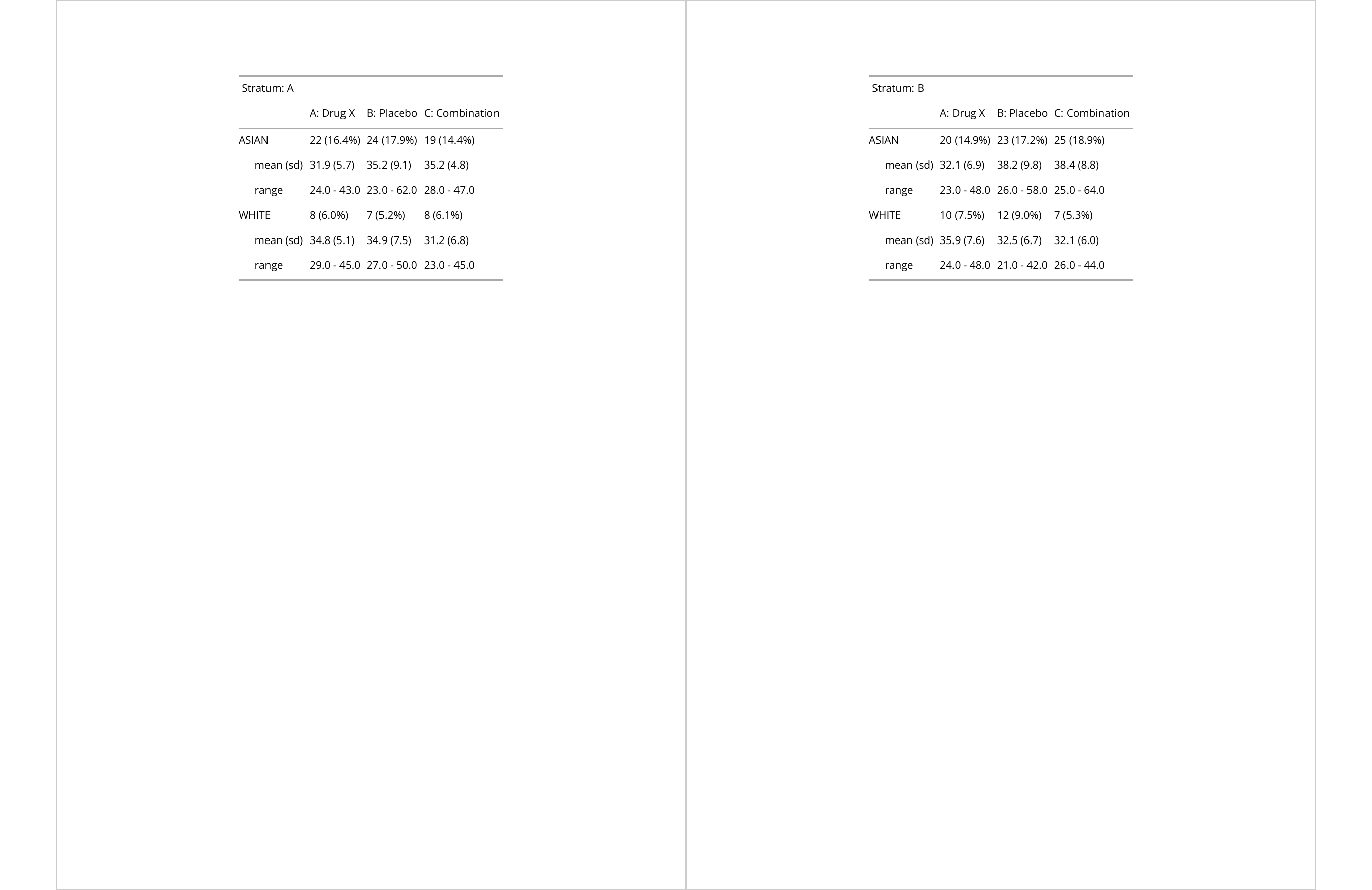
Pagination with ‘rtables’

tbl_list <- basic_table() |>
  split_cols_by("ARM") |>
  split_rows_by(
    "STRATA1", 
    split_fun = keep_split_levels(c("A", "B")), 
    page_by = TRUE, page_prefix = "Stratum") |>
  split_rows_by(
    "RACE", 
    split_fun = keep_split_levels(c("ASIAN", "WHITE"))) |>
  summarize_row_groups() |>
  analyze("AGE", afun = function(x, ...) 
    in_rows(
      "mean (sd)" = rcell(c(mean(x), sd(x)), format = "xx.x (xx.x)"),
      "range" = rcell(range(x), format = "xx.x - xx.x")
    )) |> 
  build_table(formatters::ex_adsl) |> 
  paginate_table(lpp = 20)

Now let’s use ‘officer’ to add tables into a Word document, one table per page.

doc <- read_docx()
for(name in names(tbl_list)) {
  ft <- tt_to_flextable(tbl_list[[name]]) |> 
    theme_booktabs() |> 
    font(fontname = "Open Sans")
  doc <- body_add_flextable(doc, ft)
  doc <- body_add_break(doc)
}
doc <- body_remove(doc)
print(doc, target = "assets/files/rtables-paginated.docx")

rtables-paginated

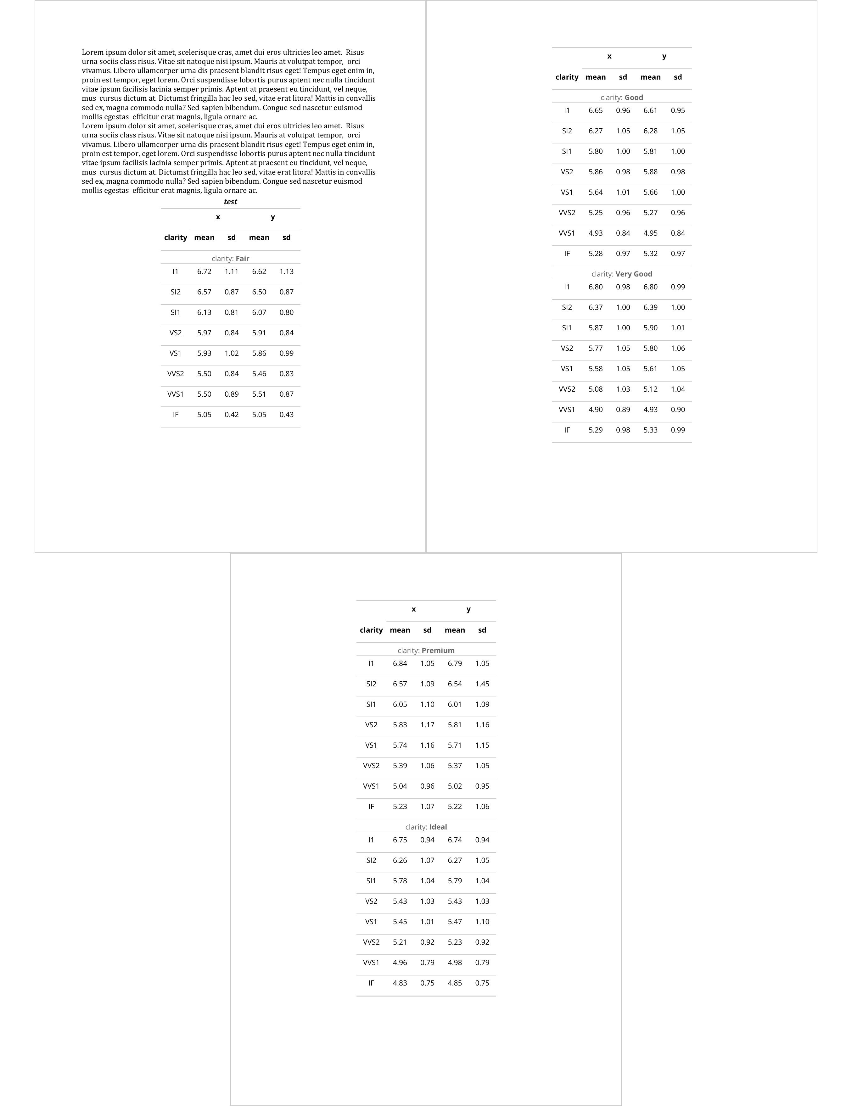
Pagination with ‘tables’

Let’s create a quick example with ‘tables’.

tab <- tabular(
  (cut*color + 1) ~ 
    (n=1) + 
    Format(digits=2)*
    (price + x)*(mean + sd), 
  data = ggplot2::diamonds)

# there are 7 'color' and 5 cut 
splits <- split(
  seq_len(7*5), 
  rep(1:5, each = 7))

Now let’s use ‘officer’ to add tables into a Word document, one table per page.

doc <- read_docx()
for(spl in splits) {
  ft <- as_flextable(tab[spl,], spread_first_col = TRUE)
  doc <- body_add_flextable(doc, ft)
  doc <- body_add_break(doc)
}
doc <- body_remove(doc)
print(doc, target = "assets/files/tables-paginated.docx")

tables-paginated.docx

Advanced Word features

We’re going to take a look at some of the features that go well with clinical reporting and Word file production:

  • adding computed fields
  • section management with officer.

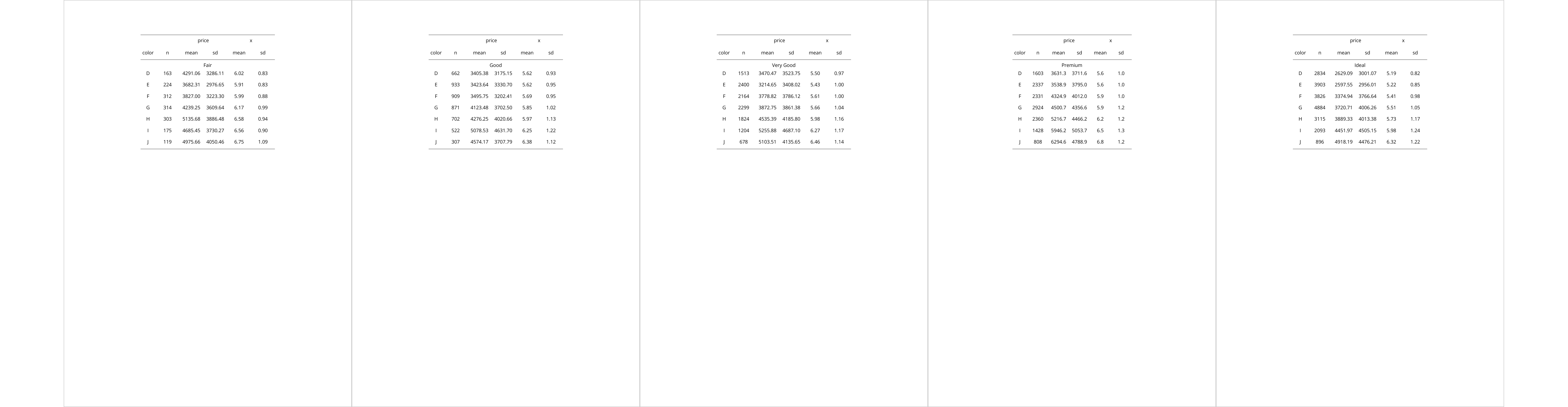
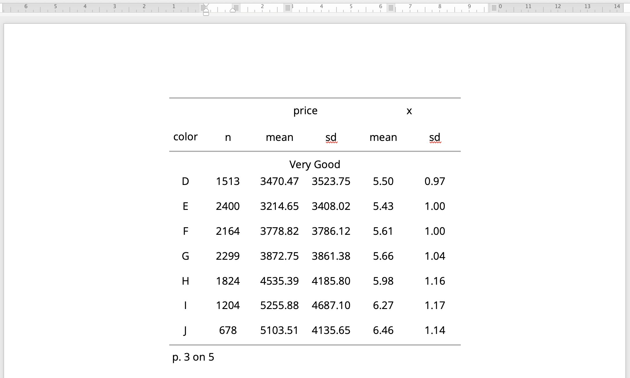
Word Computed fields and flextable

doc <- read_docx()
for (spl in splits) {
  ft <- as_flextable(tab[spl, ],
    spread_first_col = TRUE
  ) |>
    add_footer_lines(
      values =
        as_paragraph(
          "p. ",
          as_word_field(x = "Page", width = .05),
          " on ", as_word_field(x = "NumPages", width = .05)
        )
    )
  doc <- body_add_flextable(doc, ft) |>
    body_add_break()
}
doc <- body_remove(doc) |>
  print(
    target = "assets/files/tables-fields.docx"
  )

Use section headers and footers

header_default <- 
  block_list(
    fpar(ftext("p. "), 
         run_word_field(field = "Page"),
         " on ", 
         run_word_field(field = "NumPages")))
footer_default <- 
  block_list(
    fpar(
      external_img(src = "assets/img/r-in-pharma-logo.png")))

ps <- prop_section(
  header_default = header_default,
  footer_default = footer_default)

doc <- read_docx()
for(spl in splits) {
  ft <- as_flextable(tab[spl,], 
    spread_first_col = TRUE)
  doc <- body_add_flextable(doc, ft)|> 
    body_add_break()
}
doc <- body_remove(doc) |> 
  body_set_default_section(value = ps) |> 
  print(target = "assets/files/tables-sections.docx")
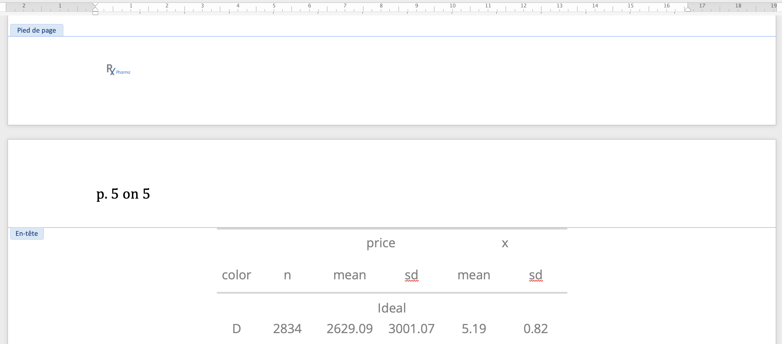
Thank you

References:

Becker, Gabriel, and Adrian Waddell. 2023. Rtables: Reporting Tables. R package version 0.6.3. https://CRAN.R-project.org/package=rtables.
Gohel, David, and Panagiotis Skintzos. 2023. Flextable: Functions for Tabular Reporting. R package version 0.9.3. https://CRAN.R-project.org/package=flextable.
Murdoch, Duncan. 2023. Tables: Formula-Driven Table Generation. R package version 0.9.17. https://dmurdoch.github.io/tables/.