News from ggiraph

ggiraph, what is it?

The ggiraph package lets you work with ggplot and produce interactive graphics. The number of features is low and ggiraph usage is simple. The three features to be aware of are:

• ability to animate points, polygons or lines,
• ability to display tooltips when mouse is over these elements,
• ability to select elements when the graphic is shwon in a shiny application.

An example with cats and meows

An illustration will help those who never used ggiraph… We will plot the distribution of cats and dogs among pets in the United States. We will display a tooltip, animate the bars and the click will trigger a dog or cat sound.

First, let’s define two JavaScript objects. these are medias that will be played when a bar will be clicked.

var ouahouah = new Audio("/media/uhauha.ogg" ) ;
var meow = new Audio("/media/Meow.ogg" ) ;

Next, we need to prepare the data for ggplot. The following code import data and create a table with repartition of cats and dogs for each state.

library(ggiraph)
library(tidyverse)

# curl download file from github ----
xlfile <- tempfile()
curl::curl_download(
  url = paste0(
    "https://github.com/davidgohel/budapestbi2017/",
    "blob/master/docs/ggiraph/data/",
    "cats-vs-dogs.xlsx?raw=true"
  ), destfile = xlfile
)

# aggregate and prepare data for ggplot/ggiraph ----
data <- readxl::read_excel(xlfile) %>%
  select(Location, `Percentage of Dog Owners`, `Percentage of Cat Owners`) %>%
  set_names(c("location", "dog", "cat")) %>%
  gather(animal, percentage, -location) %>%
  mutate(clickjs = case_when(
    animal %in% "dog" ~ "ouahouah.play();",
    animal %in% "cat" ~ "meow.play();",
    TRUE ~ "coincoin.play();"
  ), data_id = paste0(location, animal))

head(data)

We can now create a ggplot graphic, we only have to use geom_bar_interactive instead of geom_bar.

gg <- ggplot(data = data, aes(
  x = location, y = percentage, fill = animal,
  onclick = clickjs, data_id = data_id, tooltip = percentage
)) +
  geom_bar_interactive(stat = "identity") +
  theme_minimal() +
  scale_fill_manual(values = c("#FF4136", "#FFDC00")) +
  labs(title = "click on bars to play cat or dog sound!") +
  theme(axis.text.x = element_text(angle = 45, hjust = 1))

girafe(ggobj = gg, width_svg = 10, height_svg = 4) %>%
  girafe_options(ggiraph::opts_hover(css = "fill:#22222288;cursor:pointer;"))

New features

library(tibble)
library(ggiraph)
library(magrittr)

gg_point <- ggplot(
  data = mtcars,
  mapping = aes(x = wt, y = mpg, size = disp, color = as.factor(carb))
) +
  geom_point_interactive(aes(tooltip = row.names(mtcars), data_id = row.names(mtcars))) +
  scale_color_brewer(palette = "Set1", name = "carb") +
  scale_size(range = c(1, 15), name = "disp") +
  scale_x_continuous(limits = c(1, 6)) +
  scale_y_continuous(limits = c(7, 36)) +
  theme_minimal() +
  theme(legend.position = "bottom")

girafe_obj <- girafe(ggobj = gg_point) %>%
  girafe_options(
    opts_tooltip(opacity = .7),
    opts_zoom(min = .5, max = 4),
    opts_hover(css = "fill:red;stroke:white;stroke-width:2px;")
  )

JavaScript module

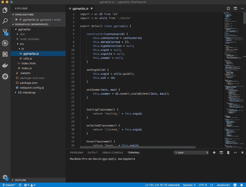
Thanks to Babel and Webpack, we have completely rewritten the JavaScript code as an ES6 module. Modularizing the application was the opportunity to clean and consolidate the code but also to better support older browsers.

This seems to have also facilitated collaboration. We received the help of Panagiotis Skintzos who did a great job of reviewing and improving the rendering (if you see a ggiraph in a shiny application from your mobile phone, praise him).

visual studio code

Next evolutions

The project is now quite stable. In the next iterations, efforts will focus on the interactive part. The work that seems to us the most motivating is the ability of having an animation on the point closest to the cursor and not only on the point under the cursor.